October 15, 2025

Reinforcement Learning for VLAs: Overview and Thoughts

Vision-Language-Action (VLA) models are quickly becoming the standard way to build general-purpose robot policies: a single neural system that can look at the world, read natural language instructions, and output low-level actions for a real robot arm . In this article, we walk through what VLAs are, why flow matching has become the dominant way to generate actions, and why combining them with Reinforcement Learning (RL) is both powerful and surprisingly hard. We then outline a concrete research proposal—FLOW-ACT (Flow Matching with Action-Critic Training)—for training flow-based VLAs with an RL critic in a way that is actually deployable on real robots.

Along the way we will focus on flow-based models (e.g. $\pi_0$ , GR-3 , $\pi_{0.5}$ ) and discuss the main challenges that arise when we try to push these models beyond pure imitation into RL-based continual improvement.

Preliminares

What are Vision-Language-Action (VLA) models?

At a high level, a VLA model takes as input:

one or more RGB images of the scene,
a natural-language instruction (e.g. “fold the towel neatly”),
robot state (joint angles, velocities, gripper state),

and outputs a sequence of robot actions—either continuous motor commands or discrete skills.

Most modern VLAs follow a similar pattern :

Backbone: a large pre-trained Vision-Language Model (VLM) that fuses images and text into a shared embedding space.
Action Expert / Head: a transformer (or similar) that consumes these embeddings plus action tokens and outputs either:
- continuous actions via a flow / diffusion model over $\mathbb{R}^d$ , or
- discrete actions / tokens that encode motion primitives or joint commands.

This modularity is key: the VLM handles semantics and spatial reasoning, while the action head specializes in robot control.

Flow-based action generation

Flow matching is a modern framework for training iterative generative models using deterministic flows instead of stochastic diffusion processes. Classical denoising diffusion models are based on stochastic differential equations (SDEs), where samples are progressively denoised by reversing a noisy Markov chain. In contrast, flow matching learns a time-dependent velocity field defining an ordinary differential equation (ODE) whose flow deterministically transports a simple base distribution (e.g., a Gaussian) into the data distribution. This leads to simpler training objectives, cheaper likelihood-free training, and faster inference, while often achieving competitive or better sample quality in practice.

Formally, let $p(x)$ be a data distribution on $\mathbb{R}^d$ . Flow matching aims to learn parameters $\theta$ of a velocity field

v_\theta(t, x) : [0, 1] \times \mathbb{R}^d \to \mathbb{R}^d

such that the induced flow $\psi_\theta(t, x)$ , defined as the solution of the ODE

\frac{d}{dt}\,\psi_\theta(t, x) = v_\theta\bigl(t, \psi_\theta(t, x)\bigr),

maps a simple base distribution at $t = 0$ (typically a standard Gaussian) into the target distribution $p(x)$ at $t = 1$ . In other words, drawing $x^0 \sim \mathcal{N}(0, I_d)$ and integrating the ODE from $t = 0$ to $t = 1$ produces a sample $x^1 = \psi_\theta(1, x^0)$ that should follow $p(x)$ .

In this article we focus on the simplest variant of flow matching based on linear paths and uniform time sampling. Given independently drawn pairs $x^0 \sim \mathcal{N}(0, I_d)$ , $x^1 \sim p(x)$ , and a time $t \sim \text{Unif}([0, 1])$ , we define the linear interpolation

x^t = (1 - t)\,x^0 + t\,x^1.

The flow matching objective trains the velocity field to point, on average, from $x^0$ toward $x^1$ along this straight-line path:

\min_\theta \mathbb{E}_{x^0, x^1, t}\bigl[\|v_\theta(t, x^t) - (x^1 - x^0)\|_2^2\bigr].

At optimum, the learned velocity field defines a flow that transports the base Gaussian into the data distribution. Sampling then amounts to numerically integrating the ODE starting from Gaussian noise; in practice, simple solvers such as Euler integration with a small number of steps are often sufficient.

For VLAs and continuous-control policies, we apply this construction in action space. Let $\mathcal{A} = \mathbb{R}^d$ denote the space of continuous actions (e.g., joint deltas or Cartesian displacements). We consider a state- and time-dependent velocity field

v_\theta(t, s, x) : [0, 1] \times \mathcal{S} \times \mathbb{R}^d \to \mathbb{R}^d,

where $s \in \mathcal{S}$ is the current robot state or observation and $x \in \mathbb{R}^d$ is a point in action space. Given demonstrations $(s, a)$ drawn from a dataset $\mathcal{D}$ , we define $x^1 = a$ , sample $x^0 \sim \mathcal{N}(0, I_d)$ and $t \sim \text{Unif}([0, 1])$ , and interpolate

x^t = (1 - t)\,x^0 + t\,x^1.

The basic flow-matching behavioral cloning objective is then

L_{\text{Flow}}(\theta) = \mathbb{E}_{\substack{s, a = x^1 \sim \mathcal{D},\\ x^0 \sim \mathcal{N}(0, I_d),\\ t \sim \text{Unif}([0, 1])}} \Bigl[\bigl\|v_\theta(t, s, x^t) - (x^1 - x^0)\bigr\|_2^2\Bigr].

The learned state-dependent velocity field induces a state-dependent flow $\psi_\theta(t, s, x)$ , which we can view as a policy. For a fixed state $s$ and noise $z \sim \mathcal{N}(0, I_d)$ , integrating the ODE from $t = 0$ to $t = 1$ with initial condition $x^0 = z$ yields an action

a = \mu_\theta(s, z) \coloneqq \psi_\theta(1, s, z).

Here, $\mu_\theta : \mathcal{S} \times \mathbb{R}^d \to \mathcal{A}$ is a deterministic mapping, but because $z$ is random we obtain an induced stochastic policy

\pi_\theta(a \mid s) \quad \text{defined by} \quad a = \mu_\theta(s, z), \; z \sim \mathcal{N}(0, I_d).

In the rest of the article we will refer to both the deterministic flow $\mu_\theta$ and the induced stochastic policy $\pi_\theta$ simply as the flow policy.

Reinforcement learning in VLAs

Most deployed VLA systems today are trained with Imitation Learning (IL) on demonstration datasets: humans teleoperate the robot or provide kinesthetic demonstrations, and the model simply learns to mimic them . However, in long-horizon, dexterous tasks (cloth folding, deformable object manipulation, bimanual skills), demonstrations can be:

noisy or inconsistent,
suboptimal or partially failing,
sparse in recovery behaviors (how to fix mistakes).

This leads to a familiar problem: the VLA can imitate “average” behavior but struggles when it needs to recover from errors or optimize success rates over time .

Why bring in Reinforcement Learning?

Reinforcement Learning provides a natural way to go beyond merely imitating an expert policy: it can learn—directly from experience—which trajectories are good or bad, use that signal to improve success rates, and keep improving autonomously over time in the real world.

learn directly from trial-and-error in the real world,
incorporate sparse success signals (task completion),
leverage human corrections as high-value signals,
gradually improve beyond the quality of the demonstration dataset .

But standard RL methods like PPO assume that the policy is a simple distribution $\pi_\theta(\mathbf{a}_t|\mathbf{s}_t)$ (e.g. a Gaussian or categorical). Flow-based VLAs instead define a generative process over actions via an ODE-like integration. Adapting policy gradients or value-based methods to this setting is non-trivial and often computationally heavy .

So, in the following sections, we will look at how this has been addressed across different paper proposals. We focus exclusively on papers that use Flow Matching to compute actions, as these represent the current state of the art.

The problem with flow matching-based policies

As previously mentioned, PPO typically assumes that the policy is a distribution $\pi_\theta(\mathbf{a}_t|\mathbf{s}_t)$ ; however, the actual flow matching process consists of learning a vector field that transports samples from an initial distribution $p_0$ to a final distribution $p_1$ . The problem with this approach is that an explicit distribution over actions cannot be obtained directly, making it difficult to apply classical RL methods based on policies or standard Q-functions.

For this reason, we will specifically discuss three key papers for this type of case: $\pi^{*}_{0.6}$ , GR-RL , and Flow Q-Learning — how they approach this problem from a general perspective, and what their weaknesses or areas for improvement are.

But first, let us clearly understand why traditional RL does not work with these types of policies.

Essentially, we need to understand the flow matching inference process. During inference, we sample from a simple distribution $p_0$ using a velocity field represented by a neural network $u_{\theta}(x,t)$ , but we do this over multiple steps — that is, we integrate over time, as illustrated in the animation below.

Flow matching inference — Euler integration from p₀ to p₁ (= a_t)

τ=0

→

τ=0.2

→

τ=0.4

→

τ=0.6

→

τ=0.8

→

τ=1

● x_τ — sample · u_θ(x,τ) — velocity field

The issue is that applying algorithms such as PPO would require backpropagating through time, which can be extremely unstable during training .

The first intuition for applying actor-critic methods would be: if we have a critic $Q(s_t,a_t)$ , then we should logically steer the flow matching process in the direction that maximizes this function; however, the difficulty lies in the actions $a_t$ . As previously noted, we would need to propagate $\nabla_{a^{\tau}_t}Q(s_t,a_t^{\tau})$ through time, which makes training extremely unstable. We will now discuss the different approaches taken in the above papers to address this challenge.

Note: The Adjoint Matching paper was recently published and addresses this problem from a different angle — it does manage to effectively propagate the gradient of the final action $Q(s_t,a_t)$ using a base model. It is a very interesting paper; unfortunately, I did not have time to review it in detail. I will update this article soon.

Proposed Solutions: A review

PI 0.6

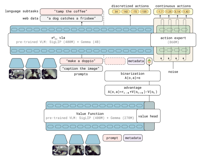
The work of $\pi^{*}_{0.6}$ addresses the same question we care about: how to improve flow-based VLAs with reinforcement learning when the policy is not a simple action distribution. Their solution rests on two main ideas: conditioning the model on whether an action is good or bad (via a scalar advantage signal), and training a separate value function that acts as a critic over trajectories. In this section we summarize their method in a formal way and spell out the equations and the iterative algorithm they use.

How they train the critic. First they train a value function $V^{\pi_{\text{ref}}}(\mathbf{o}_t, \ell)$ that estimates the expected return from observation $\mathbf{o}_t$ under the reference policy $\pi_{\text{ref}}$ , given the language instruction $\ell$ . The value function is represented as a distribution over $B$ return bins (they use $B=201$ ). For each trajectory $\tau$ in the dataset they compute the empirical return from time $t$ :

R_t(\tau) = \sum_{t'=t}^{T} r_{t'},

discretize it into a bin index $R_t^B(\tau)$ , and train the value head with cross-entropy against that target:

\min_{\phi} \mathbb{E}_{\tau \in \mathcal{D}} \left[ \sum_{\mathbf{o}_t \in \tau} H\bigl(R_t^B(\tau),\, p_{\phi}(V \mid \mathbf{o}_t, \ell)\bigr) \right]. \tag{1}

So the critic is a distributional value function trained with Monte Carlo returns from the data; the continuous value used later in the advantage is $V^{\pi_{\text{ref}}}(\mathbf{o}_t, \ell) = \sum_{b} p_{\phi}(V=b|\mathbf{o}_t,\ell)\, v(b)$ where $v(b)$ is the value of the $b$ -th bin. The reward used to compute returns is sparse and then normalized. In raw form:

r_t = \begin{cases} 0 & \text{if } t = T \text{ and success} \\ -C_{\text{fail}} & \text{if } t = T \text{ and failure} \\ -1 & \text{otherwise}, \end{cases}

where $C_{\text{fail}}$ is a large constant when the trajectory fails. They normalize this reward into $(-1, 0]$ using the longest possible trajectory length and do so per task, so that the value function and advantages live in a consistent scale. The paper notes that this is an on-policy-style estimator; while off-policy estimators could in principle do better, they found this setup simple and stable.

Conditioning on advantage. Once the value function is trained with Eq. (1), they use it to define an $n$ -step advantage and then condition the policy on it—without backpropagating through the flow. The core idea is to train the VLA with standard supervised learning but add an extra input that tells the model how good the action was in that state. The advantage is:

A^{\pi_{\text{ref}}}(\mathbf{o}_t, \mathbf{a}_t, \ell) = \mathbb{E}_{\rho_{\pi_{\text{ref}}}(\tau)} \left[ \sum_{t'=t}^{t+N-1} r_{t'} \right] + V^{\pi_{\text{ref}}}(\mathbf{o}_{t+N}, \ell) - V^{\pi_{\text{ref}}}(\mathbf{o}_t, \ell).

The only stochastic part is the sum of rewards over the next $N$ steps; the value at $t+N$ and at $t$ are given by the learned $V$ . This advantage measures how much better or worse the action $\mathbf{a}_t$ at $\mathbf{o}_t$ is compared to the average under $\pi_{\text{ref}}$ . They then condition the policy on a binary indicator $I_t = \mathbb{1}(A^{\pi_{\text{ref}}}(\mathbf{o}_t, \mathbf{a}_t, \ell) > \epsilon_\ell)$ , where $\epsilon_\ell$ is a task-dependent threshold. So the model is trained to predict actions both with and without this “good action” flag; at inference time they set $I_t = \text{true}$ so the policy always behaves as if the action were good, effectively extracting a policy that prefers high-advantage actions. The loss for this advantage-conditioned policy extraction is:

\min_{\theta} \mathbb{E}_{\mathcal{D}_{\pi_{\text{ref}}}} \Big[ -\log \pi_\theta(\mathbf{a}_t|\mathbf{o}_t, \ell) - \alpha \log \pi_\theta(\mathbf{a}_t|I_t, \mathbf{o}_t, \ell) \Big], \qquad \text{where } I_t = \mathbb{1}(A^{\pi_{\text{ref}}}(\mathbf{o}_t, \mathbf{a}_t, \ell) > \epsilon_\ell). \tag{3}

Here $\mathcal{D}_{\pi_{\text{ref}}}$ includes all data collected so far (demonstrations and autonomous rollouts); for human corrections they force $I_t = \text{true}$ . The advantage values come from the value function trained in the previous step (Eq. (1)). This formulation is closely related to classifier-free guidance: the model learns both $\pi_\theta(\mathbf{a}_t|\mathbf{o}_t, \ell)$ and $\pi_\theta(\mathbf{a}_t|I_t, \mathbf{o}_t, \ell)$ , and at deployment they condition on $I_t = \text{true}$ to bias the policy toward better actions.

Iterative data collection and the RECAP algorithm. A central feature of their method is that the whole pipeline is designed to iterate easily: they repeatedly collect new rollouts (and optionally human corrections), add them to the dataset, retrain the value function on the accumulated data, and then retrain the policy with advantage conditioning using that value function. So the “critic” is always trained on all data gathered so far, and the policy is extracted from that critic. This is summarized in their RECAP (RL with Experience and Corrections via Advantage-conditioned Policies) algorithm. In the following, $\mathcal{D}_{\text{demo}}$ is a multi-task demonstration dataset; Eq. (1) is the value loss above, and Eq. (3) is the advantage-conditioned policy loss above.

Algorithm: RECAP
Input: Multi-task demonstration dataset $\mathcal{D}_{\text{demo}}$ .

Train $V_{\text{pre}}$ on $\mathcal{D}_{\text{demo}}$ using Eq. (1).
Train $\pi_{\text{pre}}$ on $\mathcal{D}_{\text{demo}}$ using Eq. (3) and $V_{\text{pre}}$ .
For each task $\ell$ : initialize $\mathcal{D}_{\ell}$ with demonstrations for $\ell$ .
Train $V_{\ell}^{0}$ from $V_{\text{pre}}$ on $\mathcal{D}_{\ell}$ using Eq. (1).
Train $\pi_{\ell}^{0}$ from $\pi_{\text{pre}}$ on $\mathcal{D}_{\ell}$ using Eq. (3) and $V_{\ell}^{0}$ .
For $k = 1$ $k = 1$ to $K$ $K$ :
- Collect data with $\pi_{\ell}^{k-1}$ , add it to $\mathcal{D}_{\ell}$ .
- Train $V_{\ell}^{k}$ from $V_{\text{pre}}$ on $\mathcal{D}_{\ell}$ using Eq. (1).
- Train $\pi_{\ell}^{k}$ from $\pi_{\text{pre}}$ on $\mathcal{D}_{\ell}$ using Eq. (3) and $V_{\ell}^{k}$ .

So at every iteration they refit the value function on the full $\mathcal{D}_{\ell}$ (demos + all previous rollouts and corrections), then refit the policy with advantage conditioning. The figure below gives an overview of the pipeline.

GR-RL

GR-RL (ByteDance Seed) attacks the same problem—improving flow-based VLAs with reinforcement learning—but in a different way from $\pi^{*}_{0.6}$ : it uses no human corrections, treats the critic as a data filter (training only on filtered transitions), and then performs online RL by learning a noise predictor in the flow’s latent space to steer the policy toward high return. The result is a multi-stage pipeline: filter demonstrations with a learned task-progress model, augment with morphological symmetry, then run online RL to align deployment with training. We summarize the model, the filtering recipe, and the online steering procedure below.

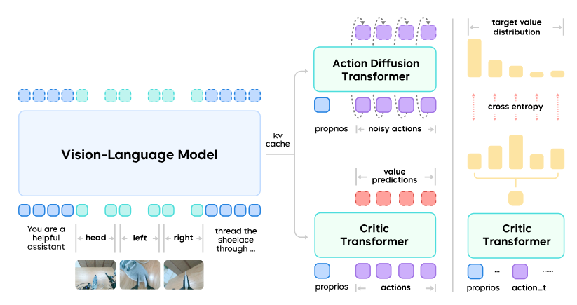
Model: policy and critic. GR-RL builds on GR-3 and uses a Mixture-of-Transformer (MoT) architecture with roughly 5B parameters. The policy $\pi_\theta$ is a vision-language-action model that outputs a $k$ -length action chunk $\mathbf{a}_t = a_{t:t+k}$ conditioned on language $l$ , observation $\mathbf{o}_t$ , and robot state $\mathbf{s}_t$ . Actions are generated by an action diffusion transformer (DiT) trained with flow matching : the policy learns a velocity field that maps noise to actions, so that sampling amounts to integrating an ODE from a base noise distribution. The critic $Q_\phi(\mathbf{o}_t, l, \mathbf{s}_t, \mathbf{a}_t)$ is a causal transformer that evaluates action chunks. Following $Q$ -chunking and distributional RL , the critic outputs a distribution over $Q$ -values (e.g. over discrete bins) instead of a single scalar. The key design choice is to bound this distribution between 0 and 1, so that the mean of the learned $Q$ -distribution naturally behaves as a task progress signal: higher value means the transition is more likely to lead to success.

Data filtering with a learned task progress evaluator

Human demonstrations in long-horizon, dexterous tasks (e.g. shoe lacing) are often suboptimal: teleoperators hesitate, make mistakes, or recover in inconsistent ways. Training with behavior cloning on all such data leads the policy to imitate these failures. GR-RL avoids that by filtering the dataset using a learned task progress model, then running behavior cloning only on the kept transitions.

Training the progress model. The progress model is the critic $Q_\phi$ , trained with offline RL (TD3+BC ) under a sparse reward. For a trajectory $\tau$ of length $T$ , the reward is defined as:

r(\mathbf{o}_t, l, \mathbf{s}_t, \mathbf{a}_t) = \begin{cases} \gamma^{T-t}\,\mathbb{I}(\tau) & t > T - k, \\ 0 & t \le T - k, \end{cases}

where $\mathbb{I}(\tau)$ is 1 if the trajectory is successful and 0 otherwise, and $\gamma$ is the discount factor. So only transitions near the end of the trajectory get a non-zero reward, and that reward is the discounted success indicator. To avoid training only on successful trajectories, they augment the dataset with failed trajectories: they mark “retry” keyframes in successful demos and create additional trajectories that stop at those keyframes (and are labeled as failures). With both successful and failed trajectories, temporal-difference learning yields a critic whose $Q$ -values reflect “how much progress toward success” each transition represents. Distributional critics (outputting a distribution over values in $[0,1]$ ) are used because they are more robust than scalar regression under sparse, noisy rewards.

Progress and filtering. Once $Q_\phi$ is trained, GR-RL defines the progress at timestep $t$ as the mean of the critic’s output distribution:

\rho_t \coloneqq \texttt{mean}\bigl(Q_\phi(\mathbf{o}_t, l, \mathbf{s}_t, \mathbf{a}_t)\bigr).

Progress tends to increase along good trajectories and drop when the demonstrator makes a mistake (e.g. misses an eyelet). A transition at $t$ is labeled suboptimal if there is a decrease in progress larger than a threshold $\delta$ in the window $\rho_{t:t+k}$ . All suboptimal transitions are removed from the dataset. The policy $\pi_\theta$ is then trained with behavior cloning on this filtered set only, so it imitates only transitions that contribute positively to progress.

Online RL: steering in noise space

A second issue is train–deployment mismatch: at inference time, the robot often uses temporal ensembling, receding-horizon control, or other smoothing, so the executed actions differ from the raw actions the policy was trained on. In dexterous, high-precision tasks this mismatch hurts. GR-RL addresses it with online RL so the policy can improve from trial-and-error with aligned execution.

Why not noise on actions? Adding noise directly to wrist poses or joint positions is ineffective for millimeter-level precision—random exploration rarely leads to success. Instead, GR-RL performs structured exploration in the latent space of the flow model ⁵⁹.

Noise predictor and critics. They add a noise predictor $\pi_{\theta'}$ (about 51.5M parameters) that, given $(\mathbf{o}_t, l, \mathbf{s}_t)$ , outputs an initial noise $\epsilon_t$ for the action DiT. So instead of always sampling $\epsilon_t \sim \mathcal{N}(0, I)$ , the policy can use $\epsilon_t \sim \pi_{\theta'}(\mathbf{o}_t, l, \mathbf{s}_t)$ to steer the flow toward high-return actions. To avoid generating out-of-distribution actions, they penalize the noise predictor when its output deviates too much from the standard normal beyond a threshold $\beta$ . They also train a critic in noise space $Q_{\phi'}(\mathbf{o}_t, l, \mathbf{s}_t, \epsilon_t)$ and distill it from the action-space critic $Q_\phi$ , so that policy gradients do not need to backpropagate through the flow model. The action-space critic $Q_\phi$ is updated with standard TD3 on real experience.

This idea is great because exploration is created by randomizing the initial noise distribution, which certainly produces different actions; however, the noise is controlled so it does not deviate too far from the original distribution or generate actions that are far outside the usual manifold.

The online objectives are:

Noise predictor (maximize value while staying close to $\mathcal{N}(0,I)$ ):

\mathcal{L}(\pi_{\theta'}) = \mathbb{E}_{(\mathbf{o}_t,l,\mathbf{s}_t)\sim\mathcal{D}} \Bigl[ -Q_{\phi'}(\mathbf{o}_t, l, \mathbf{s}_t, \epsilon_t) + c\,\max\Bigl(\frac{1}{2}\|\epsilon_t\|^2 - \beta,\; 0\Bigr) \Bigr], \qquad \epsilon_t \sim \pi_{\theta'}(\mathbf{o}_t, l, \mathbf{s}_t).

Critic in noise space (distill from $Q_\phi$ in action space):

\mathcal{L}(Q_{\phi'}) = \texttt{cross\_entropy}\Bigl( Q_{\phi'}(\mathbf{o}_t, l, \mathbf{s}_t, \epsilon_t),\; Q_\phi\bigl(\mathbf{o}_t, l, \mathbf{s}_t,\; \pi_\theta(\mathbf{o}_t, l, \mathbf{s}_t \mid \epsilon_t)\bigr) \Bigr),

where $\epsilon_t$ is sampled 50% from $\mathcal{N}(0, I)$ and 50% from $\pi_{\theta'}(\mathbf{o}_t, l, \mathbf{s}_t)$ to cover the noise space well. The policy $\pi_\theta(\cdot \mid \epsilon_t)$ denotes the action produced by the flow when initialized with noise $\epsilon_t$ .

In summary they (1) Train $Q_\phi$ with offline RL (sparse reward, successful + failed trajectories) to get a progress model. (2) Compute $\rho_t$ and filter out suboptimal transitions. (3) Train $\pi_\theta$ with behavior cloning on the filtered data and apply symmetry augmentation. (4) Optionally fine-tune $Q_\phi$ , $Q_{\phi'}$ on offline rollouts. (5) Run online RL: collect rollouts, update $\pi_{\theta'}$ and both critics; the noise predictor steers the flow toward higher return while the penalty keeps $\epsilon_t$ near $\mathcal{N}(0,I)$ . GR-RL is the first learning-based policy reported to autonomously lace a shoe (threading shoelaces through multiple eyelets), with an 83.3% success rate, combining long-horizon reasoning, millimeter-level precision, and compliant interaction with the shoe and laces .

Flow Q-Learning

Flow Q-Learning (FQL) proposes a very simple way to use flow-matching policies in offline RL without ever backpropagating through the ODE solver. Suppose we have a critic $Q_\phi(s,a)$ trained with a standard behavior-regularized actor–critic loss on a dataset $\mathcal{D}$ of transitions $(s,a,r,s')$ . The most direct idea would be to “steer” the flow policy $\pi_\theta$ by replacing the usual behavior-cloning term with the flow-matching loss $L_{\text{Flow}}(\theta)$ defined above. The actor loss would be

L_\pi(\theta) = \underbrace{\mathbb{E}_{s \sim \mathcal{D},\, a^\pi \sim \pi_\theta} \bigl[-Q_\phi(s, a^\pi)\bigr]}_{\text{Q loss}} + \underbrace{\alpha\,L_{\text{Flow}}(\theta)}_{\text{BC loss}},

so that $\pi_\theta$ is jointly pushed to maximize $Q_\phi$ and stay close to the demonstration actions through $L_{\text{Flow}}$ . The problem is that computing gradients of this loss with respect to $\theta$ requires propagating through all the ODE integration steps that produce $a^\pi = \mu_\theta(s,z)$ , i.e. full backpropagation through time, which is both unstable and expensive in practice.

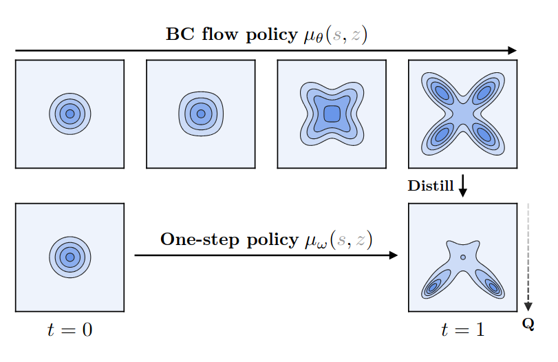
FQL’s key idea is therefore not to steer the flow policy at all. Instead, it keeps the flow policy $\mu_\theta(s,z)$ purely as a behavioral prior trained only with the flow-matching BC loss $L_{\text{Flow}}(\theta)$ , and introduces a separate one-step policy $\mu_\omega(s,z)$ that is optimized with RL. Concretely, the one-step model $\mu_\omega : \mathcal{S} \times \mathbb{R}^d \to \mathcal{A}$ takes the same noise $z \sim \mathcal{N}(0, I_d)$ and state $s$ as inputs, but outputs the action in a single forward pass, without any iterative ODE integration. Its first training signal is a distillation loss that makes it imitate the full flow policy:

L_{\text{Distill}}(\omega) = \mathbb{E}_{\substack{s \sim \mathcal{D},\\ z \sim \mathcal{N}(0, I_d)}} \Bigl[\bigl\|\mu_\omega(s,z) - \mu_\theta(s,z)\bigr\|_2^2\Bigr].

This ensures that the one-step policy initially tracks the rich action distribution produced by the BC flow model.

To inject RL, FQL simply adds a standard Q-maximization term on top of this distillation. Let $\pi_\omega(a \mid s)$ be the stochastic policy induced by $a^\pi = \mu_\omega(s,z)$ with $z \sim \mathcal{N}(0, I_d)$ . The actor loss used to train $\mu_\omega$ is

L_\pi(\omega) = \underbrace{\mathbb{E}_{s \sim \mathcal{D},\, a^\pi \sim \pi_\omega} \bigl[-Q_\phi(s, a^\pi)\bigr]}_{\text{Q loss}} + \underbrace{\alpha\,L_{\text{Distill}}(\omega)}_{\text{BC loss}}.

Intuitively, the first term pushes $\mu_\omega$ toward actions that receive high value under $Q_\phi$ , while the second term keeps it close to the BC flow policy $\pi_\theta$ . Importantly, no gradients flow through the ODE solver: the critic only ever sees one-step actions from $\mu_\omega$ , so training reduces to ordinary reparameterized policy gradients.

Mathematically, the distillation loss can be interpreted as a kind of Wasserstein behavioral regularizer. If we view $\pi_\theta(a \mid s)$ and $\pi_\omega(a \mid s)$ as the push-forwards of $z \sim \mathcal{N}(0,I_d)$ through $\mu_\theta$ and $\mu_\omega$ , then $L_{\text{Distill}}(\omega)$ upper-bounds the squared 2-Wasserstein distance $W_2^2\bigl(\pi_\omega(\cdot \mid s), \pi_\theta(\cdot \mid s)\bigr)$ in the Euclidean metric over actions. In contrast, classical offline RL methods such as TD3+BC, AWAC, or CQL regularize with KL or $\chi^2$ divergences, which are agnostic to distances in action space. FQL’s Wasserstein-style regularizer therefore encodes a more geometric notion of “staying close” to the behavioral policy, which is arguably a better inductive bias for continuous robot actions.

Putting everything together, Flow Q-Learning alternates three simple updates on minibatches from $\mathcal{D}$ : (1) update the critic $Q_\phi$ with a standard TD loss using next actions $a' = \mu_\omega(s',z)$ ; (2) update the flow policy $\mu_\theta$ with the BC flow-matching loss $L_{\text{Flow}}(\theta)$ on demonstration actions $a$ ; and (3) update the one-step policy $\mu_\omega$ with the actor loss $L_\pi(\omega)$ above. At test time, we discard the expensive ODE-based flow and deploy only the one-step policy $\pi_\omega$ , which preserves most of the expressivity of the original flow model while being cheap to evaluate and easy to train with RL.

Conclusion

There are many directions one could take if the goal is to push RL with flow-matching VLA policies beyond the current state of the art. Recent work has started to directly tackle the RL/flow interface , and even to explore one-step generative models such as Drifting Models that avoid iterative ODE integration altogether. My view is that these methods are largely complementary rather than mutually exclusive, and that the most promising future systems will likely combine ideas from several of them.

The $\pi^{*}_{0.6}$ algorithm offers a very stable way to extract a better policy from noisy data via a distributional value function over return bins and advantage conditioning. The main downside is computational: you effectively train a separate value model from scratch. A natural next step would be to reuse the representations of the underlying VLM/VLA and add an additional head—architecturally similar to the action expert—that acts as a critic. This is close in spirit to GR-RL , which already couples a large VLA policy with a distributional critic; however, its RL component is closer to progress-based data filtering and noise-space steering than to a full-fledged actor–critic update on the flow policy itself.

Flow Q-Learning takes an elegant step toward practical RL by introducing a one-step policy that distills the flow model and is trained with a Q-regularized objective, avoiding backpropagation through the ODE solver. As the authors note, this one-step parameterization can trade off some expressivity for simplicity. This is precisely where Drifting Models and Adjoint Matching become exciting: both offer ways to reason about distribution transport and credit assignment that could retain the richness of flow-based policies while enabling more direct RL-style updates, but they have not yet been thoroughly explored in the VLA setting. Investigating how to combine distributional critics, flow-based priors, and one-step or drifting-style generators for vision-language-action policies seems like a rich and very open research direction.

References

- Black, Kevin, et al. "0: A vision-language-action flow model for general robot control". arXiv preprint arXiv:2410.24164, 2025.
- Cheang, Chong, et al. "GR-3 Technical Report". arXiv preprint arXiv:2410.15570, 2024.
- Pertsch, Karl, et al. "FAST: Efficient Action Tokenization for Vision-Language-Action Models". arXiv preprint arXiv:2501.09747, 2025.
- Kim, Moo Jin, et al. "OpenVLA: An open-source vision-language-action model". arXiv preprint arXiv:2406.09246, 2024.
- Physical Intelligence, et al. "0.5: A vision-language-action model with open-world generalization". arXiv preprint arXiv:2504.16054, 2025.
- Zhao, Tony Z., and Vikash Kumar, Sergey Levine, Chelsea Finn. "Learning Fine-Grained Bimanual Manipulation with Low-Cost Hardware". arXiv preprint arXiv:2304.13705, 2023.
- Belkhale, Suneel, Yuchen Cui, and Dorsa Sadigh. "Data Quality in Imitation Learning". arXiv preprint arXiv:2306.02437, 2023.
- Li, Yunfei, et al. "GR-RL: Going Dexterous and Precise for Long-Horizon Robotic Manipulation". arXiv preprint arXiv:2512.01801, 2025.
- Physical Intelligence, et al. ": a VLA That Learns From Experience". arXiv preprint arXiv:2511.14759, 2025.
- Zhai, Shaopeng, et al. "A Vision-Language-Action-Critic Model for Robotic Real-World Reinforcement Learning". arXiv preprint arXiv:2509.15937, 2025.
- Chen, Kang, et al. ": Online RL Fine-tuning for Flow-based Vision-Language-Action Models". arXiv preprint arXiv:2510.25889, 2025.
- Murphy, Kevin. "Reinforcement Learning: An Overview". arXiv preprint arXiv:2412.05265, 2025.
- Schulman, John, et al. "Proximal Policy Optimization Algorithms". arXiv preprint arXiv:1707.06347, 2017.
- Lei, Kun, et al. "RL-100: Performant Robotic Manipulation with Real-World Reinforcement Learning". arXiv preprint arXiv:2510.14830, 2025.
- Park, Seohong, Qiyang Li, and Sergey Levine. "Flow Q-Learning". arXiv preprint arXiv:2502.02538, 2025.
- Li, Qiyang, and Sergey Levine. "Q-learning with Adjoint Matching". arXiv preprint arXiv:2601.14234, 2026.
- Fujimoto, Scott, and Shixiang Gu. "A Minimalist Approach to Offline Reinforcement Learning". Advances in Neural Information Processing Systems 34, 2021.
- Deng, Mingyang, et al. "Generative Modeling via Drifting". arXiv preprint arXiv:2602.04770, 2026.