This OpenAI paper 1 aims to improve the performance of a previous method known as Trust Region Policy Optimization (TRPO)2. It focuses on several aspects, such as reducing implementation complexity, increasing versatility by making it more compatible with general architectures, improving sampling efficiency, and providing greater training stability.

In this article, we explain in detail the key components of the proposed methodology, analyzing its most important parts. You can review the source code of the implementation at

https://github.com/NONHUMAN-SITE/ReinforcementLearning

Background

Policy Gradient Methods

As discussed in a previous article, in this type of methods, we aim to parameterize the policy directly. In that article, we demonstrated why the gradient estimators are defined in the following way:

where $A^{\pi}(a_t,s_t) = Q^{\pi}(s_t,a_t) - V^{\pi}(s_t)$ is the Advantage, which indicates how good an action is compared to the average value of all actions.

This estimator indicates the direction in which the parameters should be optimized to perform gradient ascent (since we aim to maximize the rewards). In formal terms, this translates to calculating $\nabla_{\theta}J(\pi)$ to determine the correct direction of the parameters.

The estimator is obtained empirically, i.e., by taking a small batch of finite trajectories, which is represented by the empirical average $\mathbb{E}_t[.]$ in an algorithm that alternates between optimization and sampling.

In practice, we use a loss function whose derivative coincides with this estimator so that automatic differentiation gives us the same result. Specifically, we use:

Later, we will see that, although we can perform several optimization steps over this loss function, this is not well justified and, empirically, can lead to large and destructive updates to the policy. Instead, the proposed method later regulates these effects.

Trust Region Methods

In this method, we maximize the following objective function subject to a constraint that controls the size of the policy update:

Let's analyze the objective function. Here, $\pi_{\theta_{old}}$ represents the policy before the update. Everything sampled within the trajectory and the result of $\hat{A}_t$ are determined by $\theta_{old}$. By maximizing this function:

• If $\hat{A}_t < 0$, then $\pi_{\theta_{old}}(a_t|s_t) > \pi_{\theta}(a_t|s_t)$.
• If $\hat{A}_t > 0$, then $\pi_{\theta_{old}}(a_t|s_t) < \pi_{\theta}(a_t|s_t)$.

This means that, when the advantage is negative, $\theta$ must be adjusted to reduce the probability of selecting those actions, minimizing the selection of disadvantageous actions.

On the other hand, when the advantage is positive, $\theta$ must be adjusted to increase the probability of selecting those advantageous actions.

The constraint imposed by $\mathbb{\hat{E}}_{t}[KL[\pi_{\theta_{old}}(.|s_t),\pi_{\theta}(.|s_t)]] \leq \delta$ helps control the size of the parameter update, preventing large updates that could generate instability.

Note that the term $\frac{\pi_{\theta}(a_t|s_t)}{\pi_{\theta_{old}}(a_t|s_t)}$ is not bounded. If the probability of the old policy is very small and the advantage is considerable, this value can grow too much, generating abrupt and unstable changes.

Penalty vs Constrained

The theory behind TRPO suggests reformulating this optimization process by adding a penalty term instead of a fixed constraint, i.e.:

This approach has a similar effect, since maximizing this expression naturally minimizes the divergence $KL[.]$, indicating to the parameters that they should not stray too far from the old policy $\pi_{old}$.

However, there is a key difference: the term $\beta$ controls the weight of this penalty. That is, it determines how strong the regularization effect will be.

The paper mentions that it is difficult to find a value of $\beta$ that works well in different problems, or even within the same problem, since its characteristics change as the policy improves.

Therefore, if we want a first-order algorithm that emulates the performance of TRPO, it is not enough to use this expression and then apply classic updates (i.e., use an optimizer, calculate gradients, and update $\theta$).

Clipper Surrogate Objective

Let's denote $r_t(\theta) = \frac{\pi_{\theta}(a_t|s_t)}{\pi_{\theta_{old}}(a_t|s_t)}$. Additionally, we have that $r_t(\theta_{old})=1$.

Let's define the function:

where we use CPI for Conservative Policy Iteration. As we can see, without any constraint, maximizing this function can lead to excessive policy updates. Therefore, the goal is to modify the function to penalize significant deviations from $r_t(\theta) = 1$.

The proposal is the following:

where $\epsilon$ is a hyperparameter.

The term $\operatorname{clip}(r_t(\theta),1-\epsilon,1+\epsilon)\hat{A}_t$ is present because we want to keep the ratio of probabilities bounded. Note that this ratio is equal to $1$ when $\theta = \theta_{old}$. The idea of this term is to create a confidence margin around this point, ensuring that the probability ratio remains within the interval $[1-\epsilon,1+\epsilon]$. This helps maintain policy update stability and prevents abrupt changes.

Finally, the operator $\min(.,.)$ guarantees that the objective function is a lower bound of $r_t(\theta)\hat{A}_t$. Analyzing by sections, we can observe how the behavior varies depending on the ratio value:

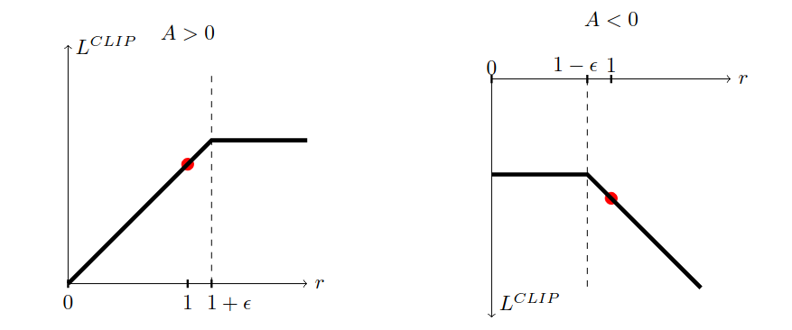
In the first figure, we observe that when the advantage is positive (i.e., the agent is performing well, $A > 0$), the ratio is bounded by $1+\epsilon$, establishing an upper limit for $\mathcal{L}^{CLIP}$ as $\mathcal{L}^{CLIP} \leq (1+\epsilon)A$. This mechanism controls parameter updates, prioritizing learning stability and avoiding drastic changes.

On the other hand, when the advantage is negative ($A < 0$), the function penalizes more strongly the agent's bad decisions. In this case, the probability ratio is kept bounded to avoid that disadvantageous actions are favored.

Adaptive KL Penalty Coefficient

Another approach is to use KL divergence as a penalty. However, in this case, we add a dynamic penalty coefficient, which adjusts to reach a target value $d_{targ}$ in each policy update. Although this method does not outperform the previous method empirically, it is mentioned in the paper as an important baseline.

The optimization function is the following:

Then, we calculate:

and update the $\beta$ value following the rule:

This means that if the KL divergence is less than the target value, the penalty decreases, allowing larger changes in the policy. Conversely, if the divergence is greater, the penalty is increased to restrict the update.

The updated $\beta$ value is used in the next policy update. With this scheme, occasional updates occur where the KL divergence significantly deviates from $d_{targ}$. However, these cases are rare, and the $\beta$ coefficient adjusts quickly. The parameters $1.5$ and $2$ were chosen heuristically, but the algorithm is not very sensitive to them. The initial value of $\beta$ is another hyperparameter, but its impact is minimal in practice because the algorithm adjusts quickly.

Algorithm

The proposed algorithm is based on a variant of Actor-Critic, where the policy $\pi_{\theta}(s)$ and the value function $V_{\theta}(s)$ share parameters. To train this type of neural networks, the objective function must include both components. Additionally, we add an entropy term to encourage exploration, as suggested by previous works.

Entropy measures how random a probability distribution is. In the case of the policy, a higher entropy value means that the agent does not always choose the action with the highest expected reward, which encourages exploration.

The objective function is:

where $c_1$ and $c_2$ are weighting coefficients, $S$ denotes entropy, and the value function is defined as:

To train this objective function, the advantage is estimated as follows:

where:

Here, $T$ represents a fixed number of timesteps.

The algorithm follows the following procedure, as shown in the figure:

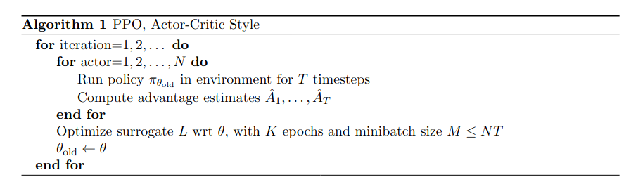
The procedure consists of using $N$ actors in parallel, each collecting data during $T$ timesteps. This generates a buffer of size $N \times T$ timesteps. Then, we use a minibatch of size $M \leq N T$ to train the model with the objective function during $K$ epochs.

Implementation

The official implementation of this algorithm is available in our Reinforcement Learning repository:

https://github.com/NONHUMAN-SITE/ReinforcementLearning/blob/main/rl/algorithm/ppo/ppo.py

However, here we will detail the most relevant parts of the implementation. Although this is a relatively simple and direct algorithm, using certain functions from our known library, PyTorch, can save us a lot of work and make the implementation more efficient.

Neural Network

As we saw earlier, this algorithm follows the actor-critic architecture, meaning that it uses two neural networks with different functions. In this case, the parameterized policy $\pi_{\theta}$ is represented by the actor, while another neural network is responsible for estimating the value of the states, i.e., $V_{\theta}(s)$. In our implementation, this is reflected as follows:

class CartPoleActorCritic(BaseActorCritic):

    def __init__(self):
        super().__init__()
        # Inicializar pesos con orthogonal initialization
        def init_weights(m):
            if isinstance(m, nn.Linear):
                nn.init.orthogonal_(m.weight, gain=1)
                nn.init.constant_(m.bias, 0)

        # Arquitectura más simple pero efectiva
        self.actor = nn.Sequential(
            nn.Linear(4, 128),
            nn.Tanh(),
            nn.Linear(128, 128),
            nn.Tanh(),
            nn.Linear(128, 2),
            nn.Softmax(dim=-1)
        )
        
        self.critic = nn.Sequential(
            nn.Linear(4, 128),
            nn.Tanh(),
            nn.Linear(128, 128),
            nn.Tanh(),
            nn.Linear(128, 1)
        )
        
        self.actor.apply(init_weights)
        self.critic.apply(init_weights)

        self.optimizer = torch.optim.Adam([
            {'params': self.actor.parameters(), 'lr': 2.5e-4},
            {'params': self.critic.parameters(), 'lr': 1e-3}
        ])

We can separate both neural networks and assign each its own optimization parameters, since PyTorch offers this flexibility.

Collect Data

Although the paper mentions that data collection should be done in parallel using $N$ actors, we have opted for this configuration, as we will later implement a mechanism that allows us to perform this computation in parallel. The main function of this module is to collect data within the buffer and then reuse them multiple times when training over these timesteps.

Other implementations often use two neural networks for the policy, often calling one of them as policy_old; however, we consider that this is not necessary, since all collected data is recorded before performing backpropagation. Nevertheless, there are two key points to keep in mind:

• Calculation of Advantage $A_t$ with GAE: This step is crucial, since it provides the reward signal to the model. If the estimation is not performed correctly, the model will not learn effectively. Its implementation can be a bit complex, since, after storing all reward values, it is necessary to consider two factors: independent trajectory segmentation and terminal state detection.

• Storing actions in the buffer: This step is essential for correctly estimating the ratio

This point will be developed in more detail in the next section.

    def parallel_recollect(self):
        '''
        Implementation of GAE (Generalized Advantage Estimation)
        '''
        for _ in range(self.cfg_algorithm.N_actors):

            state = self.env.reset()

            states   = []
            logprobs = []
            rewards  = []
            dones    = []
            values   = []
            actions  = []
            
            for t in range(self.cfg_algorithm.T_steps):

                action, logprob, value = self.model.act(state, with_value_state=True)
                
                next_state, reward, done, truncated, info = self.env.step(action)

                done = done or truncated
                
                states.append(state)
                logprobs.append(logprob)
                rewards.append(reward)
                dones.append(done)
                values.append(value)
                actions.append(action)
                state = next_state
                
                if done:
                    state = self.env.reset()
                        
            # Calculating GAE
            advantages = []
            last_advantage = 0
            last_value = values[-1]
            
            for t in reversed(range(len(rewards))):
                if dones[t]:
                    delta = rewards[t] - values[t]
                    last_advantage = delta
                else:
                    delta = rewards[t] + self.cfg_algorithm.gamma * last_value - values[t]
                    last_advantage = delta + self.cfg_algorithm.gamma * self.gae_lambda * last_advantage
                
                advantages.insert(0, last_advantage)
                last_value = values[t]
            
            advantages = torch.tensor(advantages, device=self.device)
            values = torch.tensor(values, device=self.device)

            V_targ = advantages + values
            
            for t in range(self.cfg_algorithm.T_steps):
                self.buffer.add((states[t],actions[t], logprobs[t], advantages[t], V_targ[t]))

Loss Function

New Log Probs

As we saw earlier, storing actions is a fundamental step, since to estimate the ratio

we must calculate it in terms of the taken actions. That is, this ratio represents the probability of having taken a certain action with the new policy in relation to the probability of having taken that same action with the old policy.

Therefore, we should not recalculate the actions, since this would generate an incorrect result and divert the optimization of $\theta$ in the wrong direction, as we analyzed in the previous sections.

To perform this calculation efficiently in both continuous and discrete action spaces, we use the torch.distributions library. This allows us to obtain the probability distribution in both cases and directly calculate the logarithm of the probabilities given the actions, which makes the implementation simpler, faster, and more efficient.

       #CLIP LOSS
        if self.env.is_continuous:
            action_mean = self.model.actor_forward(old_states)
            cov_matrix = torch.diag(self.model.action_var).unsqueeze(0)
            dist = torch.distributions.MultivariateNormal(action_mean, cov_matrix)
            new_logprobs = dist.log_prob(old_actions)
        else:
            probs = self.model.actor_forward(old_states)
            dist = torch.distributions.Categorical(probs)
            new_logprobs = dist.log_prob(old_actions)

The only thing to keep in mind is that, in the continuous case, we need an additional hyperparameter: self.model.action_var. This represents the variance that our model will have when sampling actions. This variable must decrease as training progresses to produce actions that are more deterministic. Additionally, this factor influences exploration and exploitation. In our code, we implemented a linear decay of this value.

Function

Beyond this detail, the loss function is quite simple, since PyTorch provides several tools to directly implement different parts of the algorithm, as shown below. An important aspect, although sometimes overlooked, is the sign of the loss. As we saw earlier, the goal is to maximize the estimator through gradient ascent; however, this is equivalent to performing gradient descent with the sign of the estimator inverted.

    def get_loss(self, sample):

        old_states, old_actions, old_logprobs, old_A_t, old_V_targ = sample

        #CLIP LOSS
        if self.env.is_continuous:
            action_mean = self.model.actor_forward(old_states)
            cov_matrix = torch.diag(self.model.action_var).unsqueeze(0)
            dist = torch.distributions.MultivariateNormal(action_mean, cov_matrix)
            new_logprobs = dist.log_prob(old_actions)
        else:
            probs = self.model.actor_forward(old_states)
            dist = torch.distributions.Categorical(probs)
            new_logprobs = dist.log_prob(old_actions)

        ratio = torch.exp(new_logprobs - old_logprobs.detach())
        clip_ratio = torch.clamp(ratio, 1 - self.cfg_algorithm.eps_clip, 1 + self.cfg_algorithm.eps_clip)

        clip_loss = torch.min(ratio * old_A_t, clip_ratio * old_A_t)


        #ENTROPY LOSS
        entropy_loss = dist.entropy()

        #VALUE LOSS
        value_states = self.model.critic_forward(old_states).squeeze()
        value_loss = self.mse_loss(old_V_targ, value_states)
        value_loss = value_loss

        #TOTAL LOSS
        loss = clip_loss - self.cfg_algorithm.vf_coef * value_loss + self.cfg_algorithm.entropy_coef * entropy_loss
        loss = -loss.mean()
        
        return loss

Results

Time to make BRRRR with the GPUs! In this section, we train the neural network on several simple and well-defined environments from the Gymnasium library. In particular, we train our policy on four different environments: CartPole, LunarLander, BipedalWalker, and CarRacing (Discrete). Below, we present several videos showing the policy performance in each of them.

All these models, and many more, are available for download in our Hugging Face repository

https://huggingface.co/NONHUMAN-RESEARCH.

References

1. J. Schulman, F. Wolski, P. Dhariwal, A. Radford, y O. Klimov, "Proximal Policy Optimization Algorithms," OpenAI

2. Schulman, John, Sergey Levine, Philipp Moritz, Michael I. Jordan, Pieter Abbeel. “Trust Region Policy Optimization”. 2015.