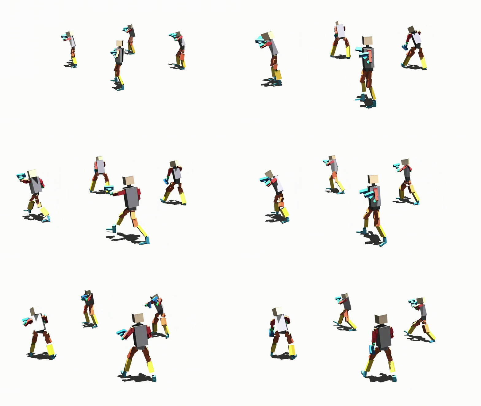
Repository: https://github.com/leoperezz/OptimalEmbodiment

Before discussing the idea, it is worth noting that many recent works have focused on robotic manipulation tasks, while comparatively few have been published on loco-manipulation. At the same time, recent research has shown that we can scale data collection by using egocentric human videos directly, with EgoScale 1 being the most promising work so far. From this, two questions arose:

• How can we scale this for full-body control tasks as well?
• What would be the perfect embodiment to absorb human movement data?

In this article, we will explore the latter, without considering hands for now, since they are a complex topic on their own; for a great discussion on dexterous hands, I highly recommend the Origami Robotics blog 2. The core idea I propose is that, given a human motion dataset, we can use the randomization technique from XHugWBC 3 to find the most effective embodiment for imitating human movement. This applies to both joints and links. Additionally, the goal is to establish a metric to estimate how optimal different existing robots are for learning from this data.

Generally speaking, this algorithm should be able to perform two things:

$$\text{Optimal Embodiment} + \text{Data} \to \text{URDF}$$

The following sections explain the process to achieve this.

Randomization

Ideally, we need an exploration algorithm; for this, we require not only a sampling method but also a morphological state space where we can sample physically plausible bodies. For this purpose, we follow the paper 3, which introduces the concept of Physics-Consistent Randomization.

Mathematical Representation of the Robot

3 starts from a template robot and defines a vector of morphological parameters:

$$\kappa = [\kappa_{\text{link}}, \kappa_{\text{joint}}] \in \mathbb{R}^N,$$

where:

• $\kappa_{\text{link}} \in \mathbb{R}^{10 n_b}$ groups the inertial parameters of the $n_b$ rigid bodies (links). Each link $i$ has:

  $$\kappa^i = [m, h_x, h_y, h_z, I_{xx}, I_{yy}, I_{zz}, I_{xy}, I_{xz}, I_{yz}]^\top \in \mathbb{R}^{10},$$

  where $m$ is the mass, $\mathbf{h} = [h_x, h_y, h_z]^\top = m \mathbf{c}$ is the first moment of mass (mass times center of mass), and $I_{\cdot\cdot}$ encodes the rotational inertia matrix $\bar{I}$ relative to the body frame origin. In other words, $\kappa_{\text{link}}$ describes how heavy each link is, where its center of mass is located, and how mass is distributed around it.

• $\kappa_{\text{joint}} \in \mathbb{R}^{13 n_d}$ groups the parameters of the $n_d$ joints. Each joint $i$ connects a parent and a child link via:

  $$\kappa_j^i = [p_x, p_y, p_z, \phi, \theta, \psi, a_x, a_y, a_z, q_{\min}, q_{\max}, \dot{q}_{\max}, \tau_{\max}]^\top \in \mathbb{R}^{13},$$

  where $\mathbf{p} = [p_x, p_y, p_z]$ is the joint position in the parent frame, $\mathbf{e} = [\phi, \theta, \psi]$ is its orientation (e.g., in Euler angles), $\mathbf{a} = [a_x, a_y, a_z]$ is the axis of movement, and $q_{\min}, q_{\max}, \dot{q}_{\max}, \tau_{\max}$ are its position, velocity, and torque limits. Essentially, $\kappa_{\text{joint}}$ describes where the hinges are, how they are oriented, which way they rotate, and their physical limits.

Naively randomizing morphologies would correspond to sampling:

$$\kappa' = \kappa + \Delta \kappa, \quad \Delta \kappa \sim \mathcal{D}_{\text{morph}},$$

but this can break physical consistency (e.g., negative masses or non-positive-definite inertia matrices). Therefore, 3 first reparameterizes the link and joint space into coordinates where adding noise is safer.

Reparameterizing the Link Space

We first derive a physics-consistent randomization solution for the link space, which mainly consists of inertial parameters

Definition 3.1 (Physics-Consistent Inertial Parameters). A rigid body's inertial parameters $\kappa_{\text{link}}$ are said to be physics-consistent if its pseudo-inertia matrix:

$$\mathbf{J} = \begin{bmatrix} \Sigma & \mathbf{h}^\top \\ \mathbf{h} & m \end{bmatrix} \qquad (2)$$

is symmetric positive definite, where:

$$\Sigma = \tfrac{1}{2} \operatorname{Tr}(\bar{\mathbf{I}})\mathbf{I} - \bar{\mathbf{I}}.$$

This condition compactly captures that mass must be positive, the center of mass must be realizable, and the inertia matrix must originate from a physically possible mass distribution.

Lemma 3.2 (Cholesky Factorization). If $\mathbf{J} \succ 0$, it admits a Cholesky decomposition:

$$J = LL^\top,$$

with $L$ being lower triangular. Any plausible pseudo-inertia matrix can be written this way. A naive randomization method would be to perturb $L$:

$$L' = L + \epsilon, \quad \epsilon \sim \mathcal{D}, \qquad J' = L' L'^\top.$$

Lemma 3.3 (Affine Transformation). If we apply an affine transformation to the rigid body coordinates, $x' = E x$, and scale the mass density $\rho' = \beta^2 \rho$, the pseudo-inertia transforms as:

$$J' = U J U^\top, \qquad U = \beta E.$$

This is derived from the integral form of $J$:

$$J = \int_V q q^\top \rho(x) \, dV, \quad q = [x^\top, 1]^\top.$$

Substituting the coordinate change yields that the new pseudo-inertia is exactly $U J U^\top$. Combining Lemmas 3.2 and 3.3 results in:

$$J' = (U L)(U L)^\top,$$

which suggests that perturbing $J$ in a physically consistent manner is equivalent to perturbing its factorization $L$ via an affine transformation $U$ associated with reasonable geometric scaling and deformations.

Geometric interpretation

Lemma 3.2 suggests a tempting randomization strategy: if $\mathbf{J} = \mathbf{L}\mathbf{L}^\top$, then perturb $\mathbf{L}$ and rebuild $\mathbf{J}$:

$$\mathbf{L}' = \mathbf{L} + \epsilon, \quad \epsilon \sim \mathcal{D}, \qquad \mathbf{J}' = \mathbf{L}' \mathbf{L}'^\top.$$

However, to understand which perturbations are meaningful (and how to parameterize them cleanly), it helps to view them through rigid-body geometry. In this context, an affine transformation can be thought of as a linear map that includes rotations and anisotropic rescalings (plus the associated homogeneous-coordinate machinery).

Lemma 3.3 states that under an affine coordinate change $x' = E x$ together with a density scaling $\rho' = \beta^2 \rho$, the pseudo-inertia transforms as:

$$\mathbf{J}' = \mathbf{U}\mathbf{J}\mathbf{U}^\top, \qquad \mathbf{U} = \beta \mathbf{E}.$$

Combining this with $\mathbf{J} = \mathbf{L}\mathbf{L}^\top$ yields:

$$\mathbf{J}' = \mathbf{U}\mathbf{L}\mathbf{L}^\top\mathbf{U}^\top = (\mathbf{U}\mathbf{L})(\mathbf{U}\mathbf{L})^\top.$$

So, perturbing the pseudo-inertia $\mathbf{J}$ can be interpreted as perturbing its Cholesky factor $\mathbf{L}$ via left-multiplication by a geometrically meaningful transform $\mathbf{U}$. If we want to match the naive perturbation $\mathbf{L}' = \mathbf{L} + \epsilon$ with an affine-induced one $\mathbf{L}' = \mathbf{U}\mathbf{L}$, we can write:

$$\begin{aligned} \mathbf{U}\mathbf{L} &= \mathbf{L} + \epsilon \\ \mathbf{U} &= (\mathbf{L} + \epsilon)\mathbf{L}^{-1} \\ &= \mathbf{I} + \epsilon \mathbf{L}^{-1}. \end{aligned}$$

This makes the key point explicit: choosing a random perturbation $\epsilon$ implicitly defines a random affine-like transform $\mathbf{U}$. The reparameterization in Lemma 3.4 is designed to sample such transforms in a controlled, interpretable way, while guaranteeing $\mathbf{J}' \succ 0$.

Lemma 3.4 (Bijective Map $\mathbb{R}^{10} \leftrightarrow U$). Instead of sampling $U$ directly, 3 constructs a bijective map between matrices $U$ and an "explainable" vector of dimension 10:

$$\theta_{\text{inert}} = [\alpha, d_1, d_2, d_3, s_{12}, s_{23}, s_{13}, t_1, t_2, t_3]^\top \in \mathbb{R}^{10}.$$

The corresponding matrix is written as:

$$\mathbf{U} = e^{\alpha} \begin{bmatrix} e^{d_1} & s_{12} & s_{13} & t_1 \\ 0 & e^{d_2} & s_{23} & t_2 \\ 0 & 0 & e^{d_3} & t_3 \\ 0 & 0 & 0 & 1 \end{bmatrix}.$$

With this construction, we obtain a bijective map from inertial parameters to a vector in $\mathbb{R}^{10}$ and vice versa. Randomizing the link space is reduced to:

1. Sampling $\theta_{\text{inert}} \in \mathbb{R}^{10}$ within bounded ranges.
2. Reconstructing $U$ from $\theta_{\text{inert}}$.
3. Calculating $J' = U J U^\top$ and, from there, the new parameters $\kappa'_{\text{link}}$.

This procedure ensures that $J'$ remains positive definite, meaning the new link remains physically realizable.

Reparameterizing the Joint Space

For the joints, 3 starts from the decomposition:

$$\kappa_{\text{joint}} = [p_x, p_y, p_z] \oplus [\phi, \theta, \psi] \oplus [a_x, a_y, a_z] \oplus [q_{\min}, q_{\max}, \dot{q}_{\max}, \tau_{\max}],$$

which can be interpreted as:

• Position $p$: where the joint (and thus the child link) is located relative to the parent link, controlling lengths and the global geometry of the robot.
• Orientation $(\phi, \theta, \psi)$: how the joint frame is oriented—i.e., how the "hinge" is placed relative to the parent body (defining the configuration zero).
• Rotation Axis $a$: in which direction the movement acts (e.g., if a door opens to one side or the other).
• Limits and Actuation: intervals $[q_{\min}, q_{\max}]$, maximum velocity $\dot{q}_{\max}$, and maximum torque $\tau_{\max}$ that characterize the actuator's physical capability.

Joint Space Randomization. In real systems, these parameters are constrained by the robot's own dynamics and construction. 3 proposes:

1. Randomizing the rotation axis $\mathbf{a}$ in key joints (e.g., the hips) to synthesize kinematically distinct yet reasonable configurations.
2. Randomizing position $\mathbf{p}$ within bounds depending on the distance to the link's center of mass, avoiding impossible geometries.
3. Scaling limits and torques consistently with total mass, so that control behavior remains comparable between morphologies with different masses.
4. Choosing joint types (revolute or fixed) in some cases, allowing certain DoFs to be locked or activated depending on the sample.

The result is a new set $\kappa'_{\text{joint}}$ that respects geometric and inertial constraints while exploring a rich family of joint configurations. In short, on the joint side we are essentially randomizing within a set of predefined intervals that are chosen to be reasonably valid.

For more details on the values/ranges explored, see the appendix in 3.

Joint Space Semantic Alignment and Morphology Graphs

A key challenge in cross-embodiment is that each robot may have a different number of degrees of freedom and a different joint order. Inspired by Lin et al. (2025), 3 defines a canonical joint space of fixed dimension $N_{\max} = 32$, where each index corresponds to a joint with a well-defined semantic meaning (e.g., "left hip roll", "right knee pitch", etc.).

For a robot with $N_r \le N_{\max}$ joints and configuration $\mathbf{q}_r \in \mathbb{R}^{N_r}$, a mapping is introduced:

$$\phi_r : \mathbb{R}^{N_r} \to \mathbb{R}^{N_{\max}},$$

such that the canonical joint state $\mathbf{q}_{\text{global}}$ is constructed as:

$$\mathbf{q}_{\text{global}}[i] = \begin{cases} \mathbf{q}_r^{(j)}, & \text{if physical joint } j \text{ maps to global index } i, \\ 0, & \text{otherwise.} \end{cases}$$

In this way, all robots share the same input/output joint space for the policy, with padding on DoFs that do not exist in a specific morphology. This semantic alignment allows training a single controller over many different morphologies.

Furthermore, a graph-based description of the morphology is built upon this canonical space. Each robot is represented as a directed kinematic graph $\mathcal{G} = (\mathcal{V}, \mathcal{E})$, where:

• $\mathcal{V}$ represents the joints (nodes).
• $\mathcal{E}$ represents the rigid connections between them (edges).

From $\mathcal{E}$, an adjacency matrix $\mathbf{A} \in \{0, 1\}^{N_{\max} \times N_{\max}}$ is defined such that:

$$(\mathbf{A})_{ij} = \begin{cases} 1, & \text{if a rigid connection } (v_i, v_j) \text{ exists}, \\ 0, & \text{otherwise.} \end{cases}$$

In practice, many humanoids have parallelogram mechanisms or parallel linkages; 3 collapses them into equivalent nodes to obtain a connected, acyclic kinematic tree. This graph representation, aligned with the canonical joint space, allows our controller and the optimal embodiment algorithm to reason structurally about very different yet comparable body topologies.

References

1. Ruijie Zheng, Dantong Niu, Yuqi Xie, Jing Wang, Mengda Xu, Yunfan Jiang, Fernando Castañeda, Fengyuan Hu, You Liang Tan, Letian Fu, Trevor Darrell, Furong Huang, Yuke Zhu, Danfei Xu, Linxi Fan. "EgoScale: Scaling Dexterous Manipulation with Diverse Egocentric Human Data." arXiv, 2026.
2. Quanting Xie, Tongzhou Liao, Yonatan Bisk. "The Dexterity Deadlock." Origami Robotics Blog, February 12, 2026.
3. Yufei Xue, YunFeng Lin, Wentao Dong, Yang Tang, Jingbo Wang, Jiangmiao Pang, Ming Zhou, Minghuan Liu, Weinan Zhang. "Scalable and General Whole-Body Control for Cross-Humanoid Locomotion." arXiv, 2026.