March 10, 2025

Action Chunking Transformer

This paper titled Learning Fine-Grained Bimanual Manipulation with Low-Cost Hardware proposes two important results both at the hardware and software levels. The problem they address is that many robotic systems requiring fine manipulation include features such as precision, closed-loop feedback, and many degrees of hand-eye coordination.

Closed-loop feedback: Refers to the control strategy that the system uses as real-time feedback to continuously adjust its actions in response to changes in the environment.

Conventional robots that achieve this level of precision usually rely on advanced sensors and expensive hardware. However, if one were to develop a low-cost system, the necessary precision for fine manipulation tasks would inevitably be lost. This limits the accessibility of these systems to laboratories with large budgets and restricts their application in environments where cost is a factor to consider.

To address these challenges, the paper introduces ALOHA (A Low-cost Open-source Hardware System for Bimanual Teleoperation), a teleoperation system designed to capture human demonstrations of manipulation with high skill without the need for specialized hardware. Complementing this system, ACT (Action Chunking with Transformers) is presented, an imitation learning algorithm that allows robots to learn precise movements from visual data.

Since we will be using a different robot, the SO-ARM100, in this article we will focus solely on the learning algorithm. However, some elements such as the dimension of the action space or the number of images to process will remain constant, while in the actual implementation these are dimensions that can be modified.

You can find the details of the robot's implementation at the following link:

Implementation

Action Chunking with Transformers:

The algorithm to be developed is called Action Chunking with Transformers and it outperforms existing Imitation Learning algorithms, as will be seen later. Below, we will discuss the pipeline and some design decisions.

Pipeline

To train the ACT algorithm, we first collect human demonstrations using the robot to be used. The information collected includes the positions of the joints of the leader robot, images from the cameras, and the actions of the demonstrations. It is important to use the leader robot because, being modified, it can better capture the real intention of the human, while the follower needs to learn these dynamics through the Imitation Learning algorithm.

Observations (O) The observations taken by our policy are defined by the positions of the joints of the follower robot and the images from the camera.

In the case of the paper, they use 4 images from different cameras as observations; however, in the SO-ARM100 project, we are only considering 2 images from different cameras. In the case of the joints, in the paper, the dimension of these is 14 because they are controlling two robotic arms; in the case of SO-ARM100, this dimension is 6.

Then we train the robot to predict the sequence of future actions given the observation. Here we define the actions as the future joint positions.

Thus, in theory, ACT tries to imitate what the human operator does in each observation. These joints are managed by PID controllers within the motors.

Action Chunking

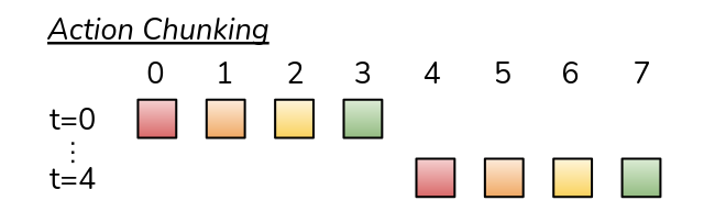
To combat the effect of compounding errors in Imitation Learning, where if our policy makes an error, it can propagate to the next state and generate an accumulated error, we modify the training in such a way that it can integrate into the pixel-to-actions policy. For this, we use the concept of action-chunking. This concept consists of modifying our policy as follows: instead of trying to predict an action at each step as

\pi(a_t|s_t)

We seek to predict the next chain of $k$ actions. Thus, our policy is posed as

\pi(a_{t:t+k}|s_t)

This is done in this way because we can reduce the effective horizon that our model has at a high frequency; where the effective horizon consists of the number of steps that our model takes to perform the task, and we refer to high frequency because we previously considered performing each action at each timestep. Thus, with action chunking, we achieve a reduction by a factor of $k$ in this effective horizon and, in addition, reduce the frequency. This allows us to reduce the compounding error, as fewer decisions are made throughout the trajectory, learning to take $k$ actions per interaction.

Temporal Ensemble

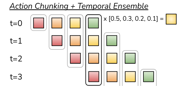
Now we will see that the native implementation of performing actions every $k$ actions is very ineffective, as it can cause the robot's movements to be very abrupt and suboptimal. Instead, we use the same concept of Action Chunking, but we add a strategy that we will call Temporal Ensemble. This strategy consists of making inferences from the model at each timestep; however, since we predict the next $k$ actions, we perform a weighted average between the effect of each previously generated action. These weights will be determined by

w_i = \frac{e^{-mi}}{\sum_{j}e^{-mj}}

where $w_0$ is the oldest action and $i$ is the relative index. Additionally, the parameter $m$ will play an important role in determining the weight of each action.

Analyzing the weights

First, note that, as the function for $w_i$ is defined, we will have the following relationship:

w_0 > w_1 > w_2 > ... > w_{k-1}

If we have only a certain number of predicted actions, say $z$ , where $1\leq z \leq k$ , we will complete the following actions $w_j=0$ with $z < j$ . Additionally, note that we will have to

\sum_{j}w_j=1

Analyzing the parameter $m$

Now let's analyze what influence and role the parameter $m$ plays. This parameter intuitively indicates how much influence the latest predicted actions will have for that timestep, as, by how the function for $w_i$ is formulated, a larger value of $m$ leads to a greater decay rate. We can see this with the following case:

\text{With} \ m=1:\ w_0=1, w_1≈0.3679, w_2≈0.1353

Let's try with a smaller value:

\text{With} \ m=0.2:\ w_0=1, w_1≈0.8187, w_2≈0.6703

We can see then that when we have a larger $m$ , the influence that the new actions have for the timestep is lower, while if $m$ is smaller, then the new actions have more influence for the current timestep.

Modeling Human Data

Note that the data from human demonstrations can be noisy; that is, for the same observation, a human may have different trajectories to solve the task or may even exhibit more stochastic behaviors, random in parts of the trajectory where precision matters less.

Example: Suppose the task is to place a cup on a shelf. Then, the movement that the arm makes to pick up the cup can be very random, and in this part, precision does not matter; however, when placing the cup is where precision matters most.

For this reason, the goal is for the policy to learn to focus on regions where precision is crucial.

To tackle this problem, it is trained as a generative model; specifically, as a Conditional Variational Autoencoder (CVAE) . This type of architecture has two important parts: the CVAE Encoder and the CVAE Decoder.

CVAE Encoder

In the following sections, we will refer to the CVAE Encoder as Encoder and the CVAE Decoder as Decoder.

The encoder within our architecture serves to train the decoder, which will be the policy, as this will be discarded at test time, that is, at the moment of inference. Mathematically, our encoder takes the information from the initial observation and carries all this information to a latent space, representing it as a variable $z$ . In this case, for faster training, the encoder takes as input the position of the joints and the sequence of target actions.

However, this process of representing the initial observation through a latent variable $z$ does not fit well with deterministic behavior, so we will obtain $z$ in a stochastic manner, that is, probabilistically. Here's the explanation.

Why a stochastic form?

Imagine the case where a human is asked to take a pencil and write their name and repeat this process a thousand times. They will realize that, although similar, each trajectory traced by the hand to write the name is not the same as the previous one; however, this similarity indicates that they belong to a probability distribution; that is, the generation of trajectories for a person to write their name is a stochastic process.

Thus, in general, if we want to imitate the demonstrations of the trajectories of movements of people when teleoperating the leader arm, we must model this process as a stochastic process so that the variable $z$ is a non-fixed representation that can capture these variations present in the demonstrations.

Thus, the mission of the encoder will not be to calculate $z$ directly, but to calculate the distribution of $z$ . In the paper, this is mathematically formalized by considering $z$ with a distribution parameterized as a diagonal Gaussian:

z \sim \prod_{i=1}^d \mathcal{N}(\mu_i,\sigma_i^2)

This represents that each component is distributed by independent parameters; that is, $z_i \sim \mathcal{N}(\mu_i,\sigma_i^2)$ . Thus, our Encoder to predict the distribution would only need to predict the mean and variance; that is, the vectors $\mu$ and $\sigma^2$ . We can then pose it as:

q_{\phi}(z∣s,a)=\mathcal{N}(z∣\mu_{\phi}(s,a),\text{diag}(\sigma_{\phi}^2(s,a)))

where $\phi$ are the parameters of the Encoder and $q$ is the distribution obtained from the observation and actions.

CVAE Decoder

The Decoder takes as input the variable $z$ and the current observations; in this case, we do include the frames of the images and the positions of the joints of the robot to predict the sequence of actions.

As we saw before, the encoder is no longer used at test time; that is, at the moment of inference, we will not have access to the variable $z$ . To resolve this, at the moment of inference, we set the variable $z=0$ . Wait, what? Yes, and now we will explain this.

$Z=0$

Since we no longer have the encoder to find the representation of $z$ at test time, we set $z=0$ , as we need a fixed value so that when performing the robot's movements, it behaves as a deterministic system.

Thus, for greater clarity, we can put it as the Encoder is responsible for learning the different styles and types of trajectories found in the demonstrations, and this is used by the Decoder to teach this type of signals; however, at the moment of inference, we need a fixed value to make the prediction, as we no longer have the information from the Encoder.

Thus, we should use a representative value, and as we know, the mean $\mu$ serves this function well. Therefore, we will seek for the mean of this variable $z$ to be equal to $0$ to use this fixed value at test time; however, how do we ensure that this mean $\mu=0$ is the most appropriate? To answer this question, we must think about how we want to train the entire model.

Thus, the model is responsible for maximizing the log-likelihood of the chunk of demonstrations. More formally, the optimization problem is as follows:

\min_{\theta}-\sum_{s_t,a_{t:t+k}\in D}\log \pi_{\theta}(a_{t:t+k}|s_t)

To minimize this function, we use the standard loss function of Variational Autoencoders, which has two terms: $\mathcal{L}_{reconst}$ and $\mathcal{L}_{reg}$ .

Reconstruction Loss

The first term is the loss function that helps us measure the distances between the actions predicted by the model and the actions from the demonstrations. For this, a standard function such as $MSE$ is used.

\mathcal{L}_{reconst} = MSE(\hat{a}_{t:t+k},a_{t:t+k})

where $\hat{a}_{t:t+k}$ are the actions predicted by the model and $a_{t:t+k}$ are the actions from the demonstrations.

Penalty Loss

Finally, we have the regularization term that will be the reason why we set $z=0$ at test time. Thus, since we seek a fixed value of $z$ to perform inference and also maintain the stability of training, we will train the parameters of the Encoder using the following penalty function:

\mathcal{L}_{reg}= D_{KL}(q_{\phi}(z|a_{t:t+k},\overline{o}_t)||\mathcal{N}(0,I))

Note: $\overline{o}_t$ refers to the observations that consist only of the joints, but without the images.

Thus, note that the regularization function uses the Kullback-Leibler divergence function. This function measures the difference between two probability distributions. In this case, the regularization function measures the difference between the distribution of $z$ parameterized by the Encoder and the Gaussian distribution with mean $0$ . This is done so that, when updating the parameters of the Encoder, the distribution of $z$ does not deviate too much from the Gaussian distribution with mean $0$ . In this way, we ensure that, although the mean of the distribution of $z$ may be different from $0$ , it will approach an approximate value due to this penalty function and, therefore, be representative of it. This guarantees that the decoder can take a good reference value and have a natural behavior when predicting actions.

Loss Function

For the final construction of the model's loss function, a hyperparameter $\beta$ is used that will measure the relevance of $z$ . In this case, we have that, the larger $\beta$ is, the less relevance will be transmitted in $z$ .

\mathcal{L} = \mathcal{L}_{reconst} + \beta\mathcal{L}_{reg}

This effect occurs because, if $\beta$ is too large, then the regularization factor will be more penalized, which would lead to the distribution of $z$ resembling more to $\mathcal{N}(0,I)$ and this would cause information to be lost, not capturing the true distribution of $z$ .

Architecture of ACT

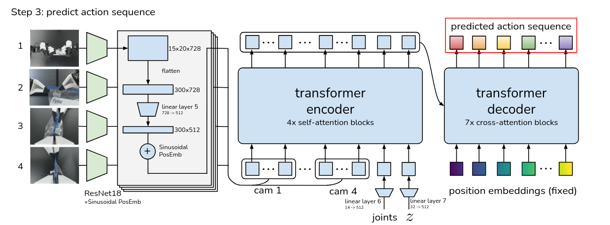
As we saw previously, the architecture of CVAE was composed of a CVAE Encoder and a CVAE Decoder. However, we must keep in mind that the same CVAE Decoder has an encoder-decoder structure. Thus, to have a better graphical visualization of the architecture, as an example, we show the following diagram of inputs and outputs:

Click to expand

CVAE Encoder

For the encoder case, an architecture similar to BERT is used. The input for training this part of the model will be composed of:

Joints (The position of the motors)
The set of $k$ actions from the demonstrations, that is, the target
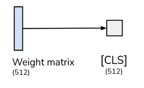
A special token [CLS] that serves to condense all the information within the corresponding output and use this to predict the mean and variance of our variable $z$ .

[CLS]

Thus, we have that our input will have a length of $k+2$ inputs. Now we will see how we will process these inputs to introduce them into our CVAE Encoder.

Initially, all must be in a common latent space. To achieve this, we will use several projections on each of the inputs so that, for the [CLS], it will be represented by a vector of dimension $512$ .

Joints

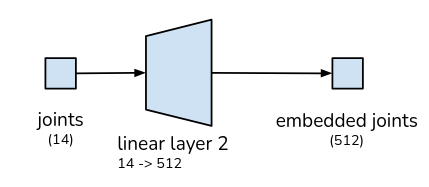
For the joints part, we have that the number of motors in the paper is $14$ , that is, two arms, so we have a vector of dimension $14$ that represents the exact position of these. Then, we need to bring them to this same dimension using a linear transformation.

Target actions

Finally, for the demonstration actions, we will have a more elaborate process. We see that we have a total of $k$ actions; that is, $k$ vectors of dimension $14$ . Thus, we use a linear transformation to bring it to the dimension of $512$ and also add the positional encoding to obtain our embedded action sequence matrix.

Final Structure

Thus, in general, we have the following graph that indicates the general structure of this CVAE Encoder.

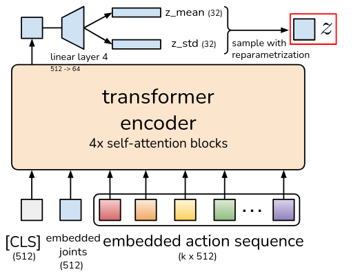
General structure of the CVAE Encoder|400x400

Note that we only use the output vector corresponding to the [CLS] vector after processing it with attention blocks and then use a linear transformation to obtain both the mean $\mu$ and the variance $\sigma^2$ . Finally, we sample $z$ to obtain our final representation.

CVAE Decoder

Now we will talk about the structure of the CVAE DECODER. Let's discuss the inputs to this part:

$z$ : It is the output obtained from the CVAE Encoder.
Image observations: These are the images collected from the trajectories. In the paper, there are 4 cameras in total.
Joints: The position of the motors in which the robot is located. In this case, there are $14$ .

Similar to the CVAE Encoder, we need to bring these inputs to a common latent space; in this case, the dimension is also $512$ .

$Z$

For the case of $z$ , we have that, since it is a vector that is in a dimension of $32$ , we need to use a linear transformation to bring it to $512$ :

z' = W . z, \ \text{where} \ W\in \mathbb{R}^{512\times 32}

Image observations

Then, for the image observations, they are in a resolution of $480 \times 640$ each. Thus, what is done first is to use the backbone of ResNet18 to process the images and convert each one from the dimension of $480 \times 640 \times 3$ to the dimension of $15 \times 20 \times 520$ . Then a flatten is performed to have it in the dimension of $300\times 512$ . Finally, positional information is added, adding a 2D positional encoding to the feature sequence.

This process is repeated for the 4 images, then we concatenate them and have a tensor that has the size of $1200\times 512$ .

Joints

For processing the joints, the current position of the motors, similarly to what was done by the CVAE Encoder, we will use a linear transformation to project it to the dimension of $512$ . Thus, we have that our current joints have a dimension of $14$ , and we use a linear layer to project it to this dimension:

J^{'}=W.J, \ \text{where} \ W\in \mathbb{R}^{512\times 14}

Final Structure

From now on, we will refer to the Encoder and Decoder, but which are within the CVAE Decoder.

Thus, in general, we have that our input will have a size of $1202\times512$ when we concatenate all our inputs. This tensor will be the input of the Encoder, then we perform a self-attention process to obtain the output of the encoder. This will have a dimension of $1202\times512$ .

Finally, we use the output of the Encoder to perform cross-attention in the Decoder. This cross-attention will have the following components as input:

Query ( $Q$ ): The query will be a fixed positional embedding. This will have the dimension of $k\times512$ , where $k$ is the number of actions to predict.
Key ( $K$ ): The key will be the output of the Encoder; that is, the matrix of $1202\times512$ added to a positional encoding.
Value ( $V$ ): The value will also be the output of the Encoder, but without adding anything.

Thus, we will have that our output will have an output of $k\times512$ , as it is only necessary to observe the multiplication of matrices, which is, in a reduced form:

(Q\times K^{T})V = (k\times512).(512\times1202).(1202\times512)

Finally, for the output, we use a linear transformation to bring this output to our action-space, which is the dimension of the motors, that is, to the dimension of $k\times 14$ .

All these multiplications are being performed at the matrix level; in reality, the batch dimension is also considered. For all this, we recommend seeing how attention mechanisms implemented in MultiHeadAttention of Pytorch work.

Now we finally have our general structure.

General structure diagram of the CVAE Decoder

Algorithms

Now we will see the algorithms for both training and inference.

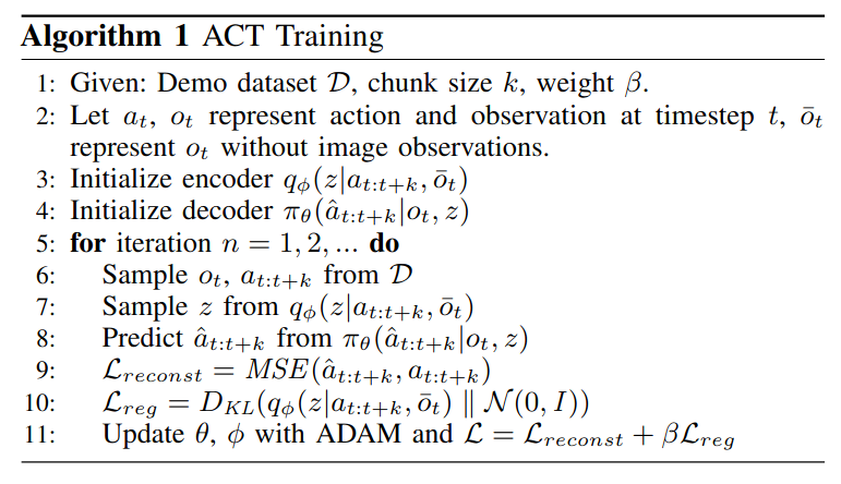
Training

The algorithm is quite straightforward. Note that the most important part has already been discussed in section 3.4.2, where we addressed the reason for the loss function and the role of $z$ within training. The most important thing we could highlight could be the structure of the dataset. As shown in the figure below, the data we need to collect must be the images, the joints, and then correlate them with the sequence of actions from the teleoperation.

Inference

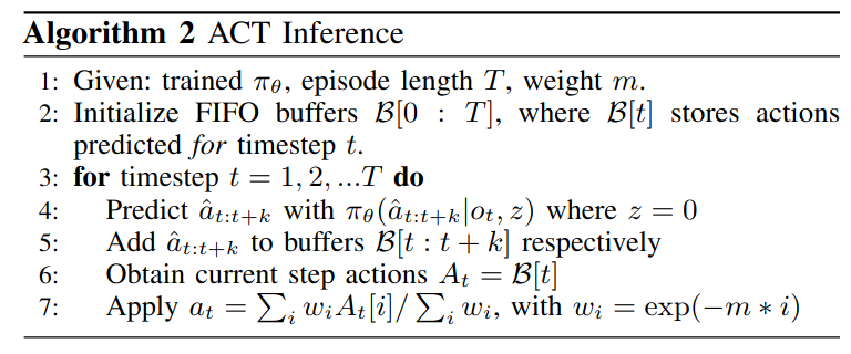
For the inference method, what stands out the most are the parts of Temporal Ensemble, which was explained in the 3.3 section. Additionally, in this section, we do not use the CVAE Encoder for inference; instead, we set $z=0$ , as it adequately represents the distribution of this latent variable, as it was trained to be so with the regularization function.

Conclusions

In this article, we explained the paper Learning Fine-Grained Bimanual Manipulation with Low-Cost Hardware that offers us a fast, low-cost, and effective method to train our robot using Imitation Learning. We covered the most important aspects and the explanation of some design decisions, from the choice of architecture to the training algorithm.

In my opinion, the most interesting parts are those of Temporal Ensemble and the choice to use a CVAE Encoder to learn the style of the trajectories from the demonstrations.

In the upcoming blogs, we will show the results and the explanation of the code for this project. Additionally, we will test new methods and architectures.

Action Chunking with Transformers:

Pipeline

Action Chunking

Temporal Ensemble

Modeling Human Data

CVAE Encoder

CVAE Decoder

Architecture of ACT

CVAE Encoder

[CLS]

Joints

Target actions

Final Structure

CVAE Decoder

ZZZ

Image observations

Joints

Final Structure

Algorithms

Training

Inference

Conclusions

References

$Z$